Like many of you, I am not a statistician but a “p-value user”. Computing p-values has become as common to me as dividing numbers or extracting their square root; however, just as division and square roots, there is usually a machine doing it for me: For some of us, “p-value users”, the p-values are still a little bit of a black box. That is why reading the “news” of p-value computation being under scrutiny is both interesting and concerning.
The following post is a summary of what I have learned about the p-value controversy and how is affecting my field of interest: bioinformatics, especially differential expression and gene set analysis.
1. A p-what?:
Let’s start by clarifying any possible confusion. Ask yourself “What is a p-value?”… Take your time until you have a good answer… Now continue… If you answered that (a) the p-value is the probability that the null hypothesis is true, or (b) it tells us if there is an effect (or a difference) in the experiment, or (c) the probability that some observations are produced by chance alone, thanks for trying, but YOU ARE WRONG! However, you are not alone in this: A review of 791 articles from 5 journals found that 51% of them wrongly interpreted the meaning of p-values and significance, usually assuming that non-significance means no effect [1].
p-values are definitively not magic numbers that decide what is true and what is not, or what is different and what is not. The technical definition of a p-value is “the probability of obtaining an effect at least as extreme as the one in your sample data, assuming the truth of the null hypothesis”. In other words, the p-value evaluates how likely are your data assuming a true null hypothesis; it is not about how likely is your hypothesis [2].
Let’s dig deeper on that definition: The null hypothesis (H0) is the statement that says that there is no relationship between two phenomena, or no difference between two groups. Usually, we want to reject H0 because we expect to find differences. Such a hypothesis corresponds to the entire population, but our data is made of samples. The samples can have differences due to sampling procedures, so we may ask how likely is that the samples reflect the population. In this context, a p-value of 0.01 indicates that, if H0 was true (if there is no difference between the groups), we still could have the observed differences/effect (or more) in 1% of the studies due to sampling error. Therefore, such a small p-value tells us that our data is actually unlikely assuming a true null. However, the p-value can’t tell you if (a) H0 is true but your sample is just unusual, or (b) H0 is false. It isn’t right to assume that small p-values imply (b) [2].
Misunderstanding the meaning of the p-values is the source of their misuse, and their misuse is the reason why some statisticians are calling for their retirement.
2. p all over the place:
The use of p-values has been questioned for a long time but, in recent years, it has been under a fiery attack. One of the most recent and influential papers was last year’s “Retire statistical significance” in Nature, signed by V. Amrhein and more than 800 other scientists [1]. However, this is just the tip of a long discussion. Just look at this list: “P values are only an index to evidence: 20th- vs. 21st-century statistical science” (Burnham and Anderson), “In defense of P values” (Murtaugh), “Understanding the new statistics: Effect sizes, confidence intervals, and meta-analysis” (Cumming), and all the books by Geoff Cumming (“Understanding the new statistics”, “Introduction to the new statistics”). Some of the papers display humorous titles such as “The earth is round (p < .05)” (Cohen) or, my favorite, “To P or not to P” (Barber and Ogle)… Nothing like a good statistical pun to make you “p” your pants…
I will explain the central criticisms to the use of p-values (and the decisions based on significance alone) based on Amrhein’s paper: The authors’ main message is to keep p-values as one of the statistical tools in the toolbox, while they urge us to abandon the current idea of statistical significance as the single way to decide if a result supports or refutes a given hypothesis. Their article provides a very illustrative example: They mention two papers studying the same phenomenon; the first paper found significance and concluded that there was support to the effect under study, while the second paper found non-significance and declared that such result was inconsistent with the first one. Amrhein et al. highlight that both studies found exactly the same effect (a risk ratio of 1.2 or a 20% increase), and the difference was that the first one was more precise than the other, with a confidence interval between 9% and 33% (p=0.0003), while the second one had an interval between -3% to 48% (p=0.091). The authors state that the observed effect is the same in both studies, so they are not in conflict, but the terms “significant” and “non-significant” can make us think that they belong to different and contradictory categories (almost as “true” and “false”). Moreover, they react against the dangers of rejecting a non-significant study, because the second study showed many individuals with serious risk increases, a situation that can’t be ignored [1].
Then how should we report our results? For the “new statistics” authors, discussing the effect size, the confidence interval, and the p-value, as a whole, is the way to go. For example: “The authors above could have written: ‘Like a previous study, our results suggest a 20% increase in risk on blah blah blah. Nonetheless, a risk difference ranging from a 3% decrease, a small negative association, to a 48% increase, a substantial positive association, is also reasonably compatible with our data, given our assumptions’. Interpreting the point estimate, while acknowledging its uncertainty, will keep you from making false declarations of ‘no difference’, and from making overconfident claims” [1]. They go even further with their recommendations: “Decisions to interpret or to publish results will not be based on statistical thresholds. People will spend less time with statistical software, and more time thinking” [1].
In words of Cumming, we are currently confronted with two different ways of statistical thinking. A “dichotomous thinking” which focuses on choosing between two mutually exclusive alternatives, and an “estimation thinking” that focuses on the values of the point and interval estimates [9]. Some authors argue that the dichotomous significance thinking should be abandoned, but there is still “value” in the p-value. “When done properly, hypothesis testing is an important precondition for estimating an effect size… Without the restraint provided by testing, an estimation-only approach will lead to overfitting of research results, poor predictions and overconfident claims” [3]. In fact, the same authors have highlighted that Fisher himself, in his 1928 book, introduced p-values just in the following way: “it is a useful preliminary before making a statistical estimate… to test if there is anything to justify estimation at all” [3].
3. All you need is size and confidence:
The current situation is a good opportunity to go back to the Statistics books and review the notions of “confidence intervals” and “effect sizes”.
A confidence interval is a range of values that we can confidently assume our true value lies in. Here is a simple example from mathisfun.com: You measure the height of 40 randomly chosen men and the result is a mean height of 175 cm with a standard deviation of 20 cm. Those are the sample mean and sd. When you compute the confidence interval, you will get a result like this: “The 95% confidence interval is 175 cm +- 6.2 cm”. That means that the true mean height is not exactly 175 cm but something between 168.8 cm and 181.2 cm. Even worst, it means that there is still a 5% chance that such interval does not include the true mean height [4]. A confidence interval is a tough reality check that reminds us to see our results in a more uncertain and probabilistic way. The following is an example of an R code to compute confidence intervals [5]:
1
2
3
4
5
6
7
mean = 5
sd = 2
n = 20
error = qnorm(0.975)*sd/sqrt(n)
left = mean - error
right = mean + error
cat ("\n", "We are 95% certain in predicting that the true mean is in the interval [", left, "-", right, "], assuming that the original random variable is normally distributed and the samples are independent.", "\n")
And here is a simple way to plot confidence intervals using ggplot [6]:
1
2
3
4
set.seed(1234)
df = data.frame(x = 1:10, mean=runif(10,1,2), lower=runif(10,0,1), upper=runif(10,2,3))
require(ggplot2)
ggplot(df, aes(x=x, y=mean)) + geom_point(size=4) + geom_errorbar(aes(ymax=upper, ymin=lower))
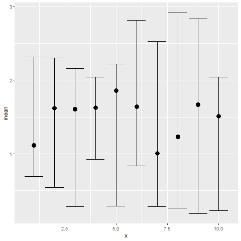
Fig 1. Confidence intervals
An effect size is an alternative to statistical significance tests to quantify the differences between two groups. Effect sizes can be quantitative values of measured phenomena, or even a ratio of values; moreover, there are standardized effect sizes such as Cohen’s d, which is the mean of the experimental group minus the mean of the control group divided by the standard deviation. Such metric is equivalent to the z-score of a normal distribution, that is, an effect size of 0.8 means that the score in the experimental group is 0.8 standard deviations above the control group. Cohen suggested that a value of d=0.2 could be interpreted as a small effect size (a real effect, just small), d=0.5 as a medium effect size, and d=0.8 as a large effect size. If the two means differ by less than 0.2 standard deviations (d<0.2), “the difference is trivial, even if it is statistically significant” [13]. I have also borrowed one simple example to explain this [7,8]. This is an example of an estimation between one sample mean and a reference value: The scores of some test by students nationwide was 516, and our group of students scored 534.78 with a sd of 93.385. The effect size would be d = 18.78 / 93.385 = 0.2. Reporting the results of this test would be something like this: A 95% confidence interval for our mean score goes from 517 to 552, while a 95% confidence interval for our effect size d goes from 0.015 to 0.386. More complex examples can be found in the above-mentioned references.
Writing this post, I have discovered a few books that teach statistics from this point of view (and also found out that they have been out there for a few years already). I didn’t have the luck to learn Statistics using such books but they are now in my to-read list [9,10]. Cumming’s “Understanding the new statistics” succintly expresses the mindset change: “Dichotomous thinking focuses on making a choice between two mutually exclusive alternatives. The dichotomous reject-or-don’t-reject decisions of NHST (null hypothesis significance testing) tend to elicit dichotomous thinking” while “Estimation thinking focuses on ‘how much’, by focusing on point and interval estimates” [9]. Estimation thinking also opens a door to meta-analytic thinking. Confidence intervals can be large for a single study but, combining evidence from multiple studies, we can get not only a better estimate but also a shorter (more precise) confidence interval. Therefore, meta-analytic thinking (and the use of meta-analysis tools such as forest plots) can be seen as an extension of estimation thinking that considers our results as one piece of information in the context of all past and future results.
4. Gene expression and estimation thinking:
When talking about gene expression studies, the most common way of quantifying differences between groups is the fold-change (or, even better, the log-fold-change). In order to get a standardized effect size we could just divide the log-fold-change by the standard deviation of the log-fold-change.
I have searched for methods that use effect sizes and confidence intervals in differential expression analysis, and I will make emphasis in one called “Topconfects” [11]. Harrison et al. start from the same place we are now: Justifying a “shift of emphasis from a dichotomous division between zero and non-zero effect size to estimating the effect size and placing confidence bounds on this estimate” [11]. The authors question the way in which we choose the resulting genes from an experiment: Most authors order the differential expression analysis results in order of p-values or false discovery rate and choose the genes above a certain cutoff value; however, we have seen that statistical significance is not the same as a biologically meaningful effect size. A first alternative could be selecting genes using a reasonable significance threshold and then ranking them (and/or further filtering) according to the log-fold-change; a second alternative would be selecting genes according to a log-fold-change threshold and then ranking according to the p-value. The authors suggest an alternative called a “confident effect size” or “confect”, which is a development of limma’s TREAT method. TREAT tests if the differential expression is greater than a given threshold (not just different from zero). Topconfects asks for a FDR and tries a range of fold changes to compute a “confect”, which is “the fold change cutoff required for TREAT to produce that set of genes at the given FDR”. Genes are then ranked by such “confident effect sizes”, and we can also obtain the confidence intervals of the fold changes. The bioconductor package also includes a series of functions called “limma_confects”, “edger_confects”, and “deseq2_confects”, which can be used to rank by confects as a final step in a limma, edgeR, or DESeq2 analysis.
Ordering the results of the differential expression analysis according to p-value and according to confect for a breast cancer dataset shows some coincidences and some differences between their gene rankings, which get more accentuated after performing GO enrichment analysis of the top genes (see paper). For the time being, I don’t have much to say about this idea, but it’s worth to keep an eye on it.
5. Gene Set Analysis and estimation thinking:
Which finally takes us to our main subject of interest. How is Gene Set Analysis making use of this way of thinking?
Here I will describe one GSA method that is using the estimation approach. It is called QuSAGE [12]. The authors highlight that existing GSA methods can’t produce confidence intervals, so they build a probability density function (pdf) of gene-set/pathway activities from which both p-values and confidence intervals can be extracted. (i) They compute the pdf of log(activities) for each gene in the treatment and control samples, and then compute the differential expression pdf for such gene; (ii) gene-set pdfs are built by combining the pdfs of the genes in the gene-set; (iii) such gene-set pdfs are then corrected by gene-gene correlation; (iv) statistical significance and confidence intervals of the gene-set activity are finally computed. After that, the authors introduce a visualization plot that includes all type of information recommended by the authors previously dicussed: Induced and repressed pathways, pathways with higher and smaller effect size, size of the confidence intervals, and the p-values, instead of the significant/non-significant dichotomy.
So let’s finish this discussion plotting a beautiful QuSAGE diagram. Let’s start by installing the R package:
1
2
3
if (!requireNamespace("BiocManager", quietly=TRUE))
	install.packages("BiocManager")
BiocManager::install("qusage")
Then, let’s follow the example on qusage’s vignette. We start with the setup:
1
2
3
4
5
6
7
8
9
10
library(qusage)
library(nlme)
data("fluExample")
data("GeneSets")

i = c(which(flu.meta$Hours==0), which(flu.meta$Hours==77))
eset = eset.full[,i]
resp = flu.meta$Condition[i]
dim(eset)
# eset[1:5,1:5]
After that, we can go with a simple case:
1
2
3
4
5
6
7
8
9
10
11
labels = c(rep("t0",17), rep("t1",17))
labels

contrast = "t1-t0"

# MSIG.geneSets = read.gmt("c2.cp.kegg.v4.0.symbols.gmt")
summary(MSIG.geneSets[1:5])
MSIG.geneSets[2]

qs.results.msig = qusage(eset, labels, contrast, MSIG.geneSets)
numPathways(qs.results.msig)
With the previous results, we can proceed to get the pathways with their log-fold-change, p-value, FDR, and a plot including all these information plus confidence intervals:
1
2
3
4
5
6
7
p.vals = pdf.pVal(qs.results.msig)
head(p.vals)
q.vals = p.adjust(p.vals, method="fdr")
head(q.vals)
qsTable(qs.results.msig, number=10)

plot(qs.results.msig)
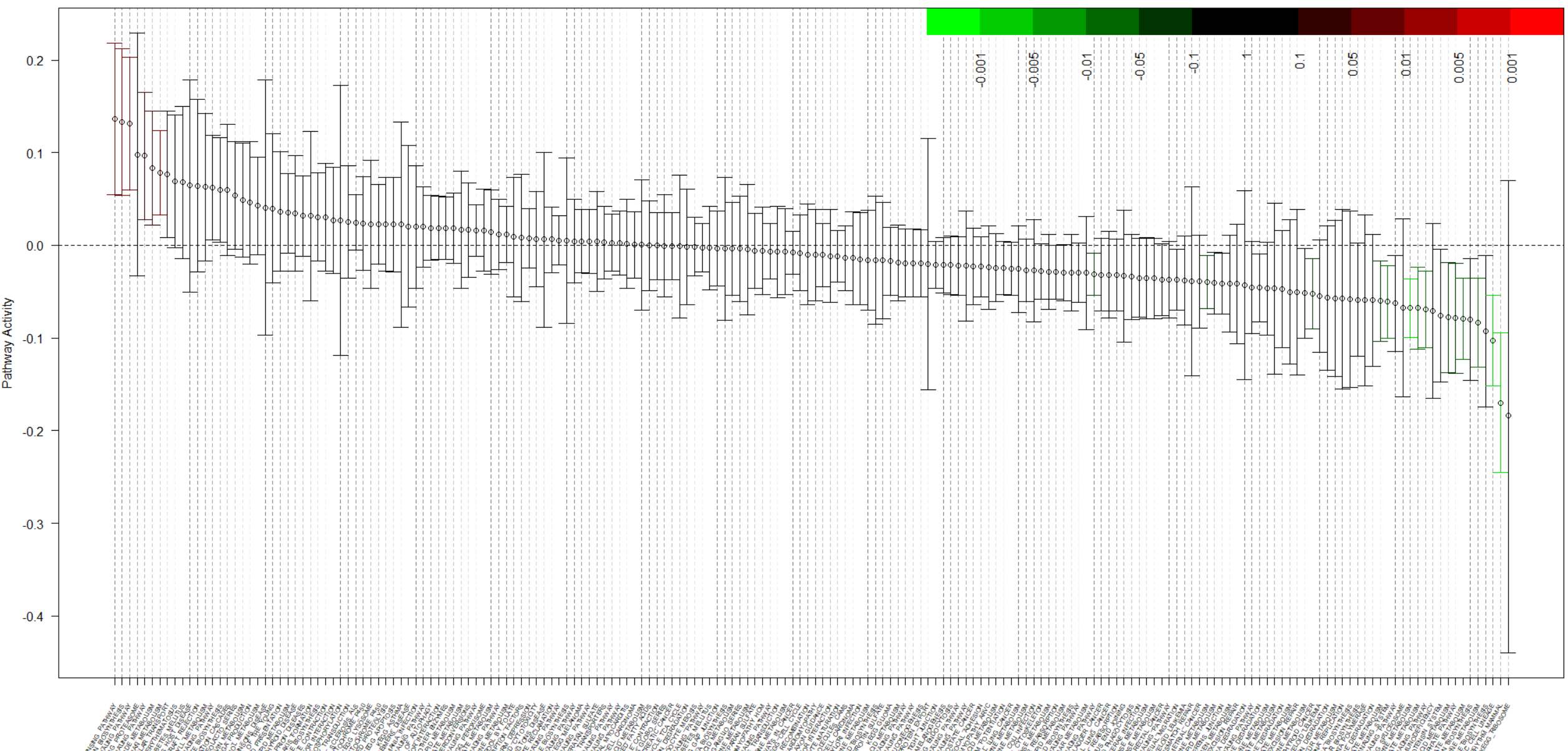
Fig 2. A QuSAGE plot
This plot is a beautiful summary of all the discussion. The x-axis contains all the gene sets, while the y axis displays the effect size (pathway activation). Every value is accompanied by its confidence interval. On the other hand, the green/red and black colors show us if the gene set is significant or not. If we are using GSA to choose one pathway to study in more detail, now we have more conceptual tools to make a decision: We want significance but also high effect size and small confidence intervals. We can explore each pathway and discover cases where significance, effect size, and confidence interval are all good, but also cases of significant pathways that show no effect, or cases of good effect size with confidence intervals that are too large (going from up-effect to no-effect to down-effect), and multiple other ways of judging our results beyond a simple p-value rank.
6. Last words:
“To p or not to p?”… The answer seems to be: “To p, to d, and to Ci”. Hopefully, in the near future, more GSA and bioinformatics tools give us the chance to judge the results according to the significance approach, but also the estimation approach; for us, “Statistics users”, such an approach constitutes both an unexpected challenge and an exciting “new” tool.
References (Recommended readings):
[1] ARMHEIN, V., et al. (2019), Retire statistical significance, Nature 567. 305-307, https://doi.org/10.1038/d41586-019-00857-9
[2] How to correctly interpret p-values, https://blog.minitab.com/blog/adventures-in-statistics-2/how-to-correctly-interpret-p-values, retrieved: 2020-05-05
[3] HAAF, J.M., et al. (2019), Retire significance, but still test hypotheses, Nature 567, 461, https://doi.org/10.1038/d41586-019-00972-7
[4] Confidence intervals, https://www.mathsisfun.com/data/confidence-interval.html, retrieved: 2020-05-05
[5] Computing confidence intervals, http://www.cyclismo.org/tutorial/R/confidence.html, retrieved: 2020-05-05
[6] Plot data with confidence intervals, https://stackoverflow.com/questions/14069629/how-can-i-plot-data-with-confidence-intervals, retrieved: 2020-05-05
[7] Effect size, https://www.leeds.ac.uk/educol/documents/00002182.htm, retrieved: 2020-05-05
[8] Effect size estimation, http://core.ecu.edu/psyc/wuenschk/StatHelp/Effect%20Size%20Estimation.pdf, retrieved: 2020-05-05
[9] CUMMING, Geoff (2012), Understanding the new statistics: Effect sizes, confidence intervals, and meta-analysis, 1st edition, Routledge.
[10] CUMMING, G. and CALIN-JAGEMAN, R. (2016), Introduction to the new statistics: Estimation, open science, and beyond, 1st edition, Routledge.
[11] HARRISON P., et al. (2019), Topconfects: a package for confident effect sizes in differential expression analysis provides a more biologically useful ranked gene list, Genome Biology, https://doi.org/10.1186/s13059-019-1674-7
[12] YAARI et al. (2013), Quantitative set analysis for gene expression: a method to quantify gene set differential expression including gene-gene correlations, Nucleic Acids Research, https://doi.org/10.1093/nar/gkt660
[13] Statistics for Psychology, Null hypothesis testing and effect sizes, https://people.bath.ac.uk/pssiw/stats2/page2/page14/page14.html, retrieved: 2020-05-05